Neural Network Research to Predict Gap Risk for Financial Assets
I set out to explore different methodologies applied to Neural Networks to predict gap risk on financial assets.
This is a blog I aim to update on a weekly basis sharing my journey for this research project.
"A bend in the road is not the end unless you fail to make the turn."Helen Keller, 1880–1968
Motivation For This Post
The inspiration for this project stems from the interest to continue learning after completing in June 2024 a 6-month Professional Certification at Imperial Business School on Machine Learning and Artificial Intelligence.
I continue experimenting with neural networks on this project. I am privileged to be guided by Ali Muhammad, who lectured me during my certification at Imperial.
In this project we use different neural network approaches to estimate gap risk on the price of financial assets, and each approach is held in a subdirectory in this repo. The projects in this repo may slightly deviate from this objective as I explore and research associated predictions that help me build towards the end goal.
This project is work in progress and this page serves as a log for this amazing journey.
Open Source Code Available
Pytorch powered project stack
Work in progress:
CNN training by encoding price time series into Gramian Angular Field (GAF) images
Application of Recurrent Neural Network with Long-short Term Memory Models
At the beginning before starting this blog post
I had a feed forward network with two convolutional layers and three fully connected layers running on a jupyter notebook. I tried to solve a regression problem and predict next day prices based on a financial time series. The model trained with Silicon Valley Bank (SIVB) and validated predictions with Silvergate Bank (SICP), both entities entered bankruptcy proceedings in 2023.
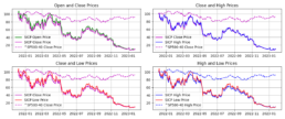
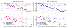
The stocks time series are encoded into images using Gramian Angular Field (GAF) to capture the similarity (GASF) or difference (GADF) between these. This approach enabled me to capture price time dependencies and enhance the explainability of results via CNNs.
Poor results on the CNN led me to start considering different architectures and study RNNs.
At this point I started posting to this blog …
Week 1
- I train and evaluate the network to solve a regression problem. I therefore evaluate R^2 metrics. However, since we predict financial asset time series prices, I am particularly interested in the relative comparison between actual and predicted values to 1 decimal place. I refer to this comparison as Threshold Accuracy:
- (torch.abs(predicted_tensor – actual_tensor)<= 0.1) / total
- The CNN results are not optimal with Threshold Accuracy in the low 20s
- I had thus started research on LSTMs and preparing a simple LSTM model to understand this better
- After meeting with Ali, I have decided that an approach that is not “fail fast” can bring benefits to my edification and eventually this research even if the results are bad
- Thus I have paused the development on the RNN and I am digging deeper on the CNN
- I have refactored the CNN from a Jupyter Notebook to python scripts and helper function modules. The model continues to yield unstable results
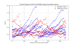
- Encoded images correlation drops to 60% whereas the actual price time series used to build these images is >99%. This is an area I need to research and understand this difference by encoding images with different parameters
- I intend to run a grid search for the above-mentioned image generation algorithm
Week 2
- I have re-trained and validated several scenarios for the CNN using GAF images. Unfortunately I had to stop because the results were hard to track. The analysis is therefore incomplete.
- The results for these simulations so far are more encouraging: validation dataset with ~60% correlation between the training/validation GAF images dataset yield [Threshold Accuracy at 1 decimal place = 44%, R^2=46%, MSE=3%].
- I still need to dig to understand the correlation between these images for different dataset but it’s clearer what hyperparameters help
- I ask my professor for guidance how to better track results and suggests mlflow. I will spend the net week setting it up.
Week 3
- I run mlflow server locally and I have setup a public mlflow server run on a docker container that servers my results from storage and the database. Unfortunately and for now, it serves from a cheap Azure SQL database so it’s not the fastest to show results
- Mlflow was particularly useful to visualize the results from encoding images with different parameters. I compared scenario results between encoding the time series into images using MarkovTransitionField vs GramianAngularField (GAF). I obtain best results (results and parameters used are stored in Mlflow gaprisk-experiment-005) with the following key encoding parameters and model parameter:
- GAF summation method
- gaf_sample_range (-1, 0.5)
- MinMax(-1,0) scaler
- dropout 0.25 to 0.5
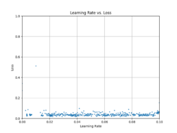
- Several runs did not converge training endlesslesly through the 10k-15k epochs. I have now added pytorch LRScheduler with Min to dynamically ratchet the learning rate down with a patience of 300 epochs. It abandons training if there is no loss improvement after 300 epochs in the case of 32×32 images.
- I hit a wall: At the best Threshold Accuracy result, the CNN gets stuck at a local minima ~0.15%. I am using multiple regularization methods:
- nn.BatchNorm1d
- Leaky ReLU
- momentum
- He kaiming weight initialization tested at 0 and range (0, 0.5)
- Dropout
- Thus I have started to search for alternative approaches that may help me reach global minima, the first being an increase the size of GAF images that may represent a larger time series cohort.
- I have also found that the performance during model training is suboptimal, my RTX 3090 Ti GPU is humming at 30-50% capacity. I suspect the root of the issue is moving tensor data to CPU to perfom interim calculations during training and log data to mlflow.
- MLflow has provided clarity in the inconsistency of results: there may be a bug in my calculation of R^2. I am going to refactor the making it more GPU optimal along with fixing this bug.
- I have added to the backlog re-running scenarios with alternative optim and loss function combinations than MSELoss and Adam.
Week 4
Week 5
- I have refactored code to keep all calculations unless necessary in the GPU. However mlflow logs require cpu metrics and this slows down training.
- I have confirmed R^2 and Threshold Accuracy calculations are correct, further confirmed with torcheval.metrics.functional.regression.r2_score. Since R^2 is calculated at 64-bit precision, it suggests poor predictions when compared to 1 decimal place Threshold Accuracy results =~50%, unlike 2 decimal place Threshold Accuracy results =~10%. Other error measures like RMSE are not as extreme.
- In relation to the GPUs low utilization rate, I have confirmed the GPUs bottleneck is not the DataLoader and for the short dataset I use, the GPU’s highest utilization for the hyper-parameters that yield the best results is when DataLoader num_workers=0, even with higher batches run (best performing batch_size=512). Disabling mlflow logging which moves data to CPU increases GPU utilization to 100% as expected. GPU utilization is 20-40% when mlflow logs.
- I have started running the Threshold Accuracy analysis for larger images
- I am now researching an embedding model suitable for univariate analysis.
Week 6
- Completed testing the network with differerent image sizes: Using the best hyperparameters and model parameters I have found that due to the short time series in this dataset, I can only run 32,64,128 image sizes. 32×32 was the most performant at 48% Threshold Accuracy and 42% R^2 for the 1 decimal place prediction calculation, whilst 2 decimal places Threshold Accuracy continues to underperform at 4%. Interestingly, to reach training loss <0.1 for these larger images, I had to remove the ReduceLROnPlateau or abandon training if convergence did not happen during training.
- Meeting with my professor this week was productive as always. I have now adjusted the backlog priority on the back of this conversation.
- Refactored to switch on/off mlflow context: back to 95% GPU utlization but no mlflow logging 🙁
Week 7
- Refactored the code to adjust the learning rate dynamically during the training and by mixing ReduceLROnPlateau Min with a LR reset rate that helps the training loss bounce off local minima with the objective of reaching global minima. Training with dropout 0.25 and weights init=0 was stuck at 0.16 min loss rate. The above mentioned strategy has helped me bring this loss to 0.02 but prediction Threshold Accuracy at 1 d.p. remains at 41%. Training with no dropout the model achieves 0.000003 loss but the lack of generalization reduces prediction accuracy by over 6%.
- I’ve enhanced the network to predict the classification for the next day price (i.e. next day price class for each window is price up or down). See Mlflow results:
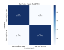
- Test Data (SIVBQ): Next day price classification class Threshold Accuracy is 95%
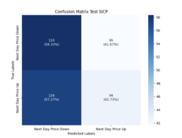
- Evaluation Data (SICP): Where next day price predicition to 1 decimal place is 41%, its corresponding next day price classification class Threshold Accuracy is 50%, and it exhibits a bearish bias reflecting the dataset used to train the model.
Week 8
- During my attendance at Unity Unite 2024 Barcelona, I came accross a discussion on the use of a wrapped adam optimizer – AdamW Cyclical Learning Rates and cosine learning rate scheduler. I implement this approach to test better generalization and smoother convergence following this implementation. The optimizer does not seem to differ much from existing Adam implementation for PyTorch, except that it separates weight decaying from batch gradient calculations. Cosine annealing scheduler with restarts allows model to converge to a (possibly) different local minimum on every restart and normalizes weight decay hyperparameter value according to the length of restart period.
- Unfortunately I observe this approach combined with loss function MSELoss does not converge to loss <0.02 and the dynamic ReduceLROnPlateau Min with a LR reset rate performs better in this regard.
Taking Stock
Weeks 1 – 8
- Training vs Evaluation time series correlation is 99% and drops to encoded GASF images = 60%
- Regression Model:
- key encoding parameters and model parameter to achieve next day price prediction best Threshold Accuracy stands at a loss <0.025
- GAF summation method
- gaf_sample_range (-1, 0.5)
- MinMax(-1,0) scaler
- dropout 0.25 to 0.5
- Adam optimizer and MSELoss function loss
- A custom pytorch ReduceLROnPlateau Min with a learning rate reset rate allows the model to reach global minima.
- The best Threshold Accuracy results are achieved via the following regularization methods to generalize:
- nn.BatchNorm1d
- Leaky ReLU
- momentum
- He kaiming weight initialization tested at 0 and range (0, 0.5)
- Dropout
- The next day price prediction results worth mentioning. We conclude minimizing the training loss erodes the benefits on model generalization.
- Min Model loss < 0.025:
- Encoded image test dataset next day prediction at 1 decimal place 67%, R^2 = 78%
- Encoded image evaluation dataset next day prediction at 1 decimal place 44%, 2 decimal places 4%, R^2 = 35%
- Min Model loss = 0.26
- Encoded image test dataset next day prediction at 1 decimal place 58%, R^2 = 78%
- Encoded image evaluation dataset next day prediction at 1 decimal place 46%, 2 decimal places 4%, R^2 = 47%
- Min Model loss < 0.025:
- key encoding parameters and model parameter to achieve next day price prediction best Threshold Accuracy stands at a loss <0.025
- Classification Model:
- Next day price higher or lower price prediction achieves global minima at function loss <0.000003 with evaluation dataset score 50%. Test dataset score 52%
Week 9
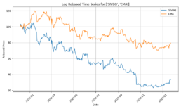
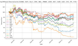
- I have completed enhancing the code to train the model with concatinated time series. Due to the price difference between stocks, I calculate rebased stock price starting at 100 for the concatinated time series and using the log return change from one time data point to the next.
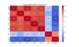
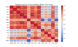
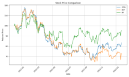
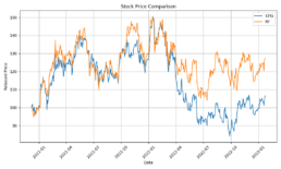
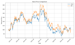
- The log-price correlation metric (image below) is not representative for our comparison purposes with highly volatile short time series because it only captures tendency but not the gamma of price – see Comerica (CMA) time series 92% correlation vs SIVBQ, whilst SIVBQ drops in price by an additional 50% in the period. Therefore I am building a dynamic time warping (DTW) metric to compare stocks similarity. This metric will also enable measuring similarity for time series of different sizes.
Week 10
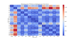
- The dynamic time warping – DTW – matrix below shows the distance for each pair of stocks, the lower the distance the greater the similarity.
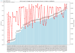
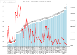
- As found in the prior week, there is a clear disconnect between log price correlation and log price DTW distance. I start investigation on this issue.
| Stock Pair Tickers | Log Price DTW Distance | Log Price Pearson Correlation |
|---|---|---|
| KEY-CFG | 461 | 0.90 |
| FITB-CFG | 632 | 0.86 |
| SIVBQ-ALLY | 1944 | 0.98 |
| FITB-ALLY | 2090 | 0.91 |
| SIVBQ-SICP | 2500 | 0.93 |
- Model predictions are far out from what would be expected when considering log price correlations. I research similarity indexes to compare encoded GAF image inputs and their respective log price time series, including:
- DTW Distance of log price series, a similarity metric which accounts for the series’ speed variation but does not translate into a higher DTW distance as long as the series are similar
- Pearson correlation: the missalignment between DTW distances and log price correlation coefficients is particularly noticeable as shown above for the FITB-CFG pair.
| Stock Pair Tickers | Log Price DTW Distance | Log Price Pearson Correlation | Encoded Image Mean Pearson Correlation | Structural Similarity (SSIM) by Tensor BxCxXxY |
|---|---|---|---|---|
| KEY-CFG | 461 | 0.90 | 0.92 | 0.7988 |
| FITB-CFG | 632 | 0.86 | 0.55 | 0.7222 |
| SIVBQ-ALLY | 1944 | 0.98 | 0.84 | 0.4821 |
| FITB-ALLY | 2090 | 0.91 | 0.70 | 0.4810 |
| SIVBQ-SICP | 2500 | 0.93 | 0.65 | 0.3705 |
- Structural Similarity Index Measure (SSIM), which extracts the structure of an image, and computed using PyTorch’s implementation, which efficiently handles multi-channel data without requiring explicit iteration over channels (unlike scikit-image library on CPU).
- Mean Squared Error (MSE) provides a pixel-wise comparison of the average squared difference between corresponding pixels.
- Cosine Similarity.
Week 11
- Model predictions are far out from what would be expected when considering log price correlations. I research similarity indexes to compare encoded GAF image inputs and their respective log price time series, including:
- DTW Distance of log price series.
- Pearson correlation: the missalignment between DTW distances and log price correlation coefficients is particularly noticeable as shown in the images in Week 10 for the FITB-CFG pair.
Week 12:
- I seek to compare last week’s similarity metrics to the neural network’s Threshold Accuracy .
- I have implemented a few more changes to train and evaluate:
- Network’s Loss Function: Taking cue from the results in this research paper, I have tested training the network with Mean Absolute Error (MAE). The paper goes further to suggest to train with a 10-day stride and a 20-day overlap between successive windows.
- I implement this function loss with pytorch as nn.L1Loss().
- In my case predictions performed better with a stride of 1. I will need to test this further as it may over-fit the data.
- I also refactored the code to a less exhaustive windowing approach than what I had, and a 25-day overlap between windows.
- Regularization: I notice the model fails to generalize with these new settings. I have substituted regularization function ReLU for Swish which I picked up about its use from this kaggle competition. The Pytorch implementation is SiLU. It improves the results, in particular evaluation R^2 but the Threshold Accuracy metric is similar to ReLUs.
- Network’s Loss Function: Taking cue from the results in this research paper, I have tested training the network with Mean Absolute Error (MAE). The paper goes further to suggest to train with a 10-day stride and a 20-day overlap between successive windows.
- I obtain Threshold Accuracy metric for divergent pairs of stocks:
| MLFlow Link | Training-Eval Stocks | DTW Distance | Input Images MSE | Input Images SSIM | Evaluation Threshold Accuracy at 0.1 (%) | R^2 (%) | Model Loss |
|---|---|---|---|---|---|---|---|
| Click Here | PWBK-OZK | 1291 | 1.97 | 0.05 | 22.2 | -0.07 | 0.010 |
| Click Here | SIVBQ-PWBK | 6038 | 2.19 | 0.05 | 16.6 | -0.22 | 0.013 |
| Click Here | ZION-KEY | 514 | 0.395 | 0.61 | 58.33 | 0.38 | 0.014 |
| Click Here | CFG-RF | 2020 | 0.375 | 0.63 | 41.66 | 0.33 | 0.015 |
| Click Here | FITB-CFG | 632 | 0.28 | 0.72 | 66.6 | 0.65 | 0.014 |
| Click Here | KEY-CFG | 460 | 0.14 | 0.8 | 72.2 | 0.85 | 0.014 |
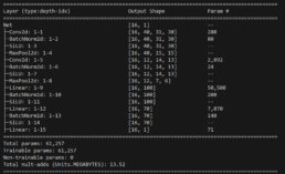
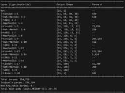
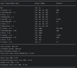
- Since both SSIM and MSE are metrics calculated on the image metrics and are consistent, I conclude a possible cause for the network’s threshold Threshold Accuracy deviation occurs because feature extraction is sub-optimal for different time series. Base on research findings, I explore adding two additional convolutional layers targeting results for the deviations I observed, I outline below the difference in the network before and after the enhancement. Unfortunately, the threshold Threshold Accuracy predictions are stlightly worse but the over performance in Threshold Accuracy for images with higher MSEs remains.
Week 13:
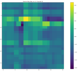
- SSIM and MSE are consistent, and their prediction Threshold Accuracy is also consistent except for pair ZION-KEY and CFG-RF. I observe the SSIM metric of the resulting feature maps captured after the last convo2d layer and fully connected layers flip: CFG-RF Feature Map SSIM < ZION-KEY Feature Map SSIM. ZION-KEY prediction Threshold Accuracy is indeed greater than CFG-RF but the Threshold Accuracy gap is over 17% (41% vs 58%).
- The higher SSIM for CFG-RF could be due to the model overfitting on features that are common but not necessarily contribute to predict stock price movements of RF.
- CFG-RF has slightly lower SSIM in the convolutional layers compared to ZION-KEY. Since convo layers are responsible for initial feature extraction, any shortcomings here may impact the quality of features passed to FC layers.
| Training-Eval Stocks | DTW Distance | Input Images MSE | Input Images SSIM | Feature Image Conv2d SSIM | Feature Image Fully Connected SSIM | Evaluation Threshold Accuracy at 0.1 (%) | Evaluation R^2 (%) | Model Loss |
|---|---|---|---|---|---|---|---|---|
| PWBK-OZK | 1291 | 1.97 | 0.05 | 0.1138 | 22.2 | -0.07 | 0.010 | |
| SIVBQ-PWBK | 6038 | 2.19 | 0.05 | 0.1099 | 16.6 | -0.22 | 0.013 | |
| ZION-KEY | 514 | 0.395 | 0.61 | 0.5708 | 0.4154 | 58.33 | 0.38 | 0.014 |
| CFG-RF | 2020 | 0.375 | 0.63 | 0.5431 | 0.5708 | 41.66 | 0.33 | 0.015 |
| FITB-CFG | 632 | 0.28 | 0.72 | 0.5966 | 0.5394 | 66.6 | 0.65 | 0.014 |
| KEY-CFG | 460 | 0.14 | 0.8 | 0.6930 | 72.2 | 0.85 | 0.014 |
Week 14:
- I set out to examine descriptive statistics for each of the layers weights and gradients. This may shed some light on weight explosion, overfitting or otherwise.
- The lower SSIM index for FC layers observed for CFG-RF pair may infer the network is struggling to learn features in the later layers. An increase in the optimizer’s adamw_weight_decay may help.
- Stepping during training for CFG-RF pair, I find:
- Training R^2 reaches 1 early on stabilizing around 0.993 indicating overfitting. I am considering re-training with dropout.
- The conv1 layer exhibits slightly asymmetrical distributions (non-zero means) that increases over epochs, suggesting that weight drift might be happening. The continued growth during training of conv1.weight_weight_std is consistent with weight drift. By contrast, the drift may be present for Conv2 during training but its weights mean converges at zero by the end of training.
- The increasing dispersion of the conv weights means may indicate that the model is learning more nuanced and specific patterns, with individual weights adjusting to fit particular training samples or features. However, and in the particular case of conv1, the combination of the continued increase in the mean (drfit) and dispersion may well be that the network is overfitting.
- Since both conv1 and conv2 gradients means oscillate around zero, the model may not be learning, except as observed by the drift on the weights, possibly idiosyncrasies rather than general patterns, leading to overfitting. An increase in the optimizer’s weight decay to penalize large weights help me prevent these from increasing.
- fc1 weights and its gradient exhibits a similar drift / overfitting behaviour to conv1. FC2 gradients means oscillate around zero which may indicate the model may not be learning at this layer.
- bn_fc2 and bn_fc2.weight_weight_mean and bn_fc2.weight_weight_std stabilize on the last 20% of training. Its weights mean ~0.8 indicates the layer is scaling inputs close to their learned distribution. Std ~0.4-0.6 indicates it allows for diverse patterns to be passed on without overly compressing feature ranges. These should hopefully help to generalize.
- bn_fc2.weight gradients fluctuate in a low range throughout training, indicating its makes small adjustments to its weights, and should help us avoid overfitting.
- fc3 shows stable weights and gradients, indicating its has converges and is well regularized.
- fc3.bias mean seems to be “offsetting” or behaving like an increasing bias shift, perhaps trying to correct or balance cnn and fc layers above it that output higher values on average than the model requires to match the observations. This raises some concern as all layers should be sharing this heavy lifting. Forcing this adjustment may be behind the SSIM degrament observed at the FC3 layer.
- Following these observationsm, I think I’ve identified as possible issue and to balance learning throughout the network
- I increase the optimizer’s weight decay to prevent weight drift (from 0.00001 to 0.001) and
- introduce dropout (from 0 to 0.4) to achieve generalization
Week 15:
- Having experimented with additional convo and FC layers in this network, I conclude convo layers learn quickly and thoroughly, possibly so much these can overfit. The lion share of the learning relies on these layers. Trying to shift this learning to the fully connected layers yields low R^2 results. For example, since in general the SSIM inputs-to-Layer Feature maps is >60% for convo layers and 25% for FC layers, and in order to balance more evenly the learning between these two layers, I took an extreme scenario where optimizer’s learning rate of convo layers is set to 0.0000001 and that for fully connected layers to 0.1. The objective was to observe if an evaluation R^2 followed an SSIM FC increase. Both train and evaluation R^2 dropped significantly. In particular, when the SSIM_FC spikes, it leads to a major drop in training R^2. On this basis I think of this network where the convo layers learns complex patterns and the FC layers serves as an offset. The challenge is the combination of these layers and the SSIMs achieved, help us generalize.
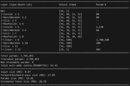
- The objective is to increase the SSIM of FC layers whilst not overfitting with too high SSIM of Convo layers. I use a simpler model (see mlflow results).
- I find SSIM Convo > 60% with SSIM FC > 50% produce evaluation R^2 >65% (fixed precision float16) and 70% at float32, eval MAE 0.108. Unfortunately, higher traininig R^2 leads to overfitting and reduces the generalization of the model for the pair Train with CFG – Evaluation with RC. Recall this pair is an outlier, in that its SSIM Input-Evaluation dataset is relatively high =0.65 but the DTW Distance is large = 2020.
- Unfortunately, none of the multiple regularization techniques used with this setup helped generalize the model when evaluated with RF stock series, but the model’s performance decreased dramatically. Other architectures tested would overfit or under perform when regularization techniques were used, making this test the best performant.
- Weights and volatility and proving to be stable during training:
- Training the model with CFG shares time series prices the training R^2 is 0.5678 and lowest cum loss 0.1458. These are the comparable results accross selected stocks by interest in DTW and SSIM against this CFG trained checkpoint.
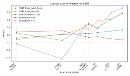
- The table reflects a clear relationship between SSIM input-to-evaluated GAF images and the model’s predictive performance. Convo SSIM feature image output to the CFG image training input is also consistent. This relationship begings to break at the FC layer feature image output level, consistent with our observation that the FC layer offsets convo layer outputs to closer predict the labels.
- Interestingly, FITB’s MAE = 0.12 > RF MAE = 0.095 and yet both prediction R^2 are pretty much the same.
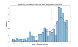
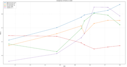
- The graph indicates the threshold where the model’s predicted values start to underperform is over 0.7.
| Eval Stock | DTW Distance To CFG | Stock Pair Images SSIM | SSIM Inputs Training-Vs-Feature Image Conv2d Eval | SSIM Inputs Training-Vs-Feature Image FC Eval | Evaluation Threshold Accuracy 1 dp (%) | Evaluation MAE | Evaluation R^2 |
|---|---|---|---|---|---|---|---|
| OZK | 1261.1 | 0.5620 | 0.5858 | 0.3172 | 50.0 | 0.1559 | 0.3140 |
| PWBK | 999.9 | 0.0565 | 0.2229 | 0.1444 | 16.66 | 0.2888 | -0.0830 |
| SIVBQ | 5443 | 0.3778 | 0.4032 | 0.3152 | 5.55 | 0.2775 | 0.0273 |
| ZION | 628.8 | 0.5414 | 0.5541 | 0.4291 | 38.88 | 0.1833 | 0.2563 |
| FITB | 632.7 | 0.72 | 0.6532 | 0.5092 | 58.33 | 0.1233 | 0.6964 |
| KEY | 514 | 0.8 | 0.7382 | 0.5067 | 44.44 | 0.1426 | 0.5724 |
| RF | 2020 | 0.6275 | 0.6176 | 0.4633 | 66.66 | 0.09514 | 0.6998 |
- I then train/evaluate with the CFG-KEY pair. A more complex model performs better with ~90% evaluation R^2 and MAE=0.0951.
| Eval Stock | DTW Distance To CFG | Stock Pair Images SSIM | SSIM Inputs Training-Vs-Feature Image Conv2d Eval | SSIM Inputs Training-Vs-Feature Image FC Eval | Evaluation Threshold Accuracy 1 dp (%) | Evaluation MAE | Evaluation R^2 |
|---|---|---|---|---|---|---|---|
| OZK | 1261.1 | 0.5620 | 0.9473 | 0.1333 | 38.88 | 0.1739 | 0.2031 |
| PWBK | 999.9 | 0.0565 | 0.9140 | 0.0914 | 16.66 | 0.3882 | -1.1904 |
| SIVBQ | 5443 | 0.3778 | 0.9392 | 0.1445 | 19.44 | 0.2596 | -0.1551 |
| ZION | 628.8 | 0.5414 | 0.9516 | 0.2111 | 38.88 | 0.1531 | 0.4448 |
| FITB | 632.7 | 0.72 | 0.9638 | 0.4490 | 63.88 | 0.0920 | 0.8599 |
| KEY | 514 | 0.8 | 0.9682 | 0.4871 | 69.44 | 0.0760 | 0.8810 |
| RF | 2020 | 0.6275 | 0.9563 | 0.3015 | 38.88 | 0.1721 | 0.0844 |
Week 16:
In-Training Learning rate Bayesian optimization experiment:
- Since changing the network’s architecture or hyperparmeters led to an overfitted model, I considered testing whether a learning rate derived via bayesian optimization with the objective function being an epoch’s training loss + an adjustment factor that primarily increased this loss for any low training-input-image-to-FullyConnected-feature-map SSIM.
- I implemented this using the GPyOpt library because it was easy to read, integrates nicely with the optimizer and was easy to test. However it had some limitations for the user to control exploration/exploitation.
- Unfortunately, the adjustment factor would not help and the model overfit (mlflow experiment)
Bettering Results – Smoothing Predictions and Architecture Optimization
- To better track on-going evaluation progress, I add onto the code evaluation after each epoch. It also facilities saving the best model on a timely basis contingent on its R^2.
- To obtain the highest evaluation R^2 I set learning rate=0.1 and adamw optimizer weight decay=0.001. But then I find the evaluation R^2 is very volatile. Iterestingly multple epochs achieve over 50% SSIM FC in ocassions peaking over 60% and 70%. Furthermore, SSIM for the Convo layers remain above 88%. We may infer from this, and hence find this encouraging, that the FC are now pulling their weight in the representation space along with the convo layers.
- See volatile now outdated mlflow graphs CFG-RF results and CFG-KEY:
- When changing the code to evaluate stepping on epochs with net.eval(), I set the net back to train() before the start of the next epoch. Since net.train() should enable regularization nn.BatchNorm and dropout, and the current dropout=0, I find that by removing batch normalization R^2 is stable and yields to the same best results. It wasn’t exactly easy to find though 🙂
- I effectively substitute batch norm for a lighter optimizer adamw weight decay = 0.0001 and gradient clipping=5 to cap backprop gradient magnitudes.
- I also find that with this setup, the cyclic scheduler works best with also a lighter base learning rate=0.001. Furthermore, since I can achieve SSIM Convo > 80% and FC > 60% I disable loss adjustments since forcing higher SSIM FC is not necessary I can avoid overfitting.
- The best evaluation results are not significantly different, but yield more stable results during training. This opens opportunities for further optimization.
- The improved results with optimized hyperparameters for CFG-KEY yielding evaluationh R^2=91% and training R^2=98.2%. SSIM and Evaluation R^2 align nicely except for anomalies SIVBQ and RF which displaces the SSIM order probably due to the their series differences captures in its DTW metrics. The peak-to-trough for this pair CFG-KEY in the period 2021-12-06 to 2023-01-25 is -44.1%.
| Eval Stock | Eval Stock Peak-to-Trough | DTW Distance To CFG | Stock Pair Images SSIM | SSIM Inputs Training-Vs-Feature Image Conv2d Eval | SSIM Inputs Training-Vs-Feature Image FC Eval | Evaluation Threshold Accuracy 1 dp (%) | Evaluation MAE | Evaluation R^2 |
|---|---|---|---|---|---|---|---|---|
| OZK | -32.9% | 1261.1 | 0.5620 | 0.2290 | 0.3537 | 47.22 | 0.1341 | 0.5069 |
| PWBK | -32.1% | 999.9 | 0.0565 | 0.1134 | 0.0730 | 25.0 | 0.2781 | -0.0373 |
| SIVBQ | -78.1% | 5443 | 0.3778 | 0.2096 | 0.2192 | 5.55 | 0.3090 | -0.4345 |
| ZION | -42.3% | 628.8 | 0.5414 | 0.2377 | 0.3881 | 44.44 | 0.1521 | 0.4482 |
| FITB | -41.4% | 632.7 | 0.72 | 0.3029 | 0.6152 | 61.11 | 0.0962 | 0.7820 |
| KEY | -44.7% | 514 | 0.8 | 0.3318 | 0.7593 | 77.77 | 0.0684 | 0.9119 |
| RF | -30.9% | 2020 | 0.6275 | 0.2618 | 0.5718 | 38.88 | 0.1505 | 0.3529 |
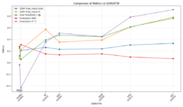
- Since we observe a certain strength of the DTW metric can have an impact on predictions, a similarity strength measured as SSIM/DTW shows a re-ordering of the pairs whilst the trend is maintained. The SSIM/DTW scale partly explains the kinked evaluation R^2 graph for ZION-OZK-RF. I believe it is unnecessary to elaborate on the patterns observed in the graph for stocks PWBK-SIVBQ, as the R^2 value is negative. Once R^2 becomes negative, its magnitude carries limited interpretive significance, as it merely indicates that the model’s performance is worse than the baseline and does not provide meaningful insights into the observed data relationships.
- The case for CFG-RF pair was more tedious. This pair has SSIM 2020.The architecture and setup that provided non-volatile R^2 led to the model overfitting and ruined evaluation R^2 improvement beyond 55% as long as the training R^2 was below 75%. Training R^2 above 75% led to evaluation R^2 <20%. Regularization techniques didn’t help – dropout, batch regularization, weight decay, clip grads.
- Therefore, in improve on the above and to increase the evaluation R^2 for the CFG-RF pair but maintain a stable training pattern, I implemented the following changes (See mlflow experiment). This achieved 70% evaluation R^2 and train R^2=0.9893:
- A more complex model
- Mainatained a learning rate = 0.001 and a higher minimum learning rate for the cyclic scheduler
- Applied regularization Norm2 to convo layers and LayerNorm to fully connected layers.
- Trained the model with the log chained time series for CFG and its most similar (DTW and SSIM) series in the set – KEY, effectively doubling the training series. Chaining tickers for larger time series training with observable tickers also opens the opportunity to experiment and generalize towards a particular target stock pair.
Longer training time series study:
- I then move on to study training the model with longer training time series in two ways:
- Extend the history of a training stock time series by a year
- Calculate the change of log prices for two stocks and concat the two, where the second attaches to the former by continuining the percentage changes
- The time series for the evaluation stocks remains at 1 year and shorter than training
- The above methodology therefore reduces SSIM and increases DTW
- I optimize the hyperparameters for CFG+KEY-RF (training series CFG+KEY in this order): I note Input image vs Evaluation SSIM metrics are not generated because the training dataset is twice larger than the evaluation dataset. Due to lower training/evaluation similarities and despite the larger training dataset, the prediction accuracy drops.
| Eval Stock | DTW Distance To CFG+KEY | Evaluation Threshold Accuracy 1 dp (%) | Evaluation MAE | Evaluation R^2 |
|---|---|---|---|---|
| OZK | 21397.6 | 47.22 | 0.1440 | 0.4563 |
| PWBK | 15704.2 | 16.66 | 0.3121 | -0.2062 |
| SIVBQ | 15832.3 | 25.0 | 0.2581 | -0.1458 |
| ZION | 8050.3 | 52.77 | 0.1413 | 0.5089 |
| FITB | 9825.1 | 27.77 | 0.1628 | 0.5917 |
| KEY | 8328.8 | 47.22 | 0.1232 | 0.7056 |
| RF | 24995.1 | 55.55 (66.66 at earlier epoch but not best eval R^2) | 0.1006 | 0.6997 |
- The table below shows the prediction results for different training and evaluation series lengths. This is generally consistent with the shorter series results and guides us to continue running predictions with shorter time series that explicitly focus on the gap region:
| Train Stock | Training Series Dates | Training Series Daycount | Train Peak-to-Trough | Eval Stock | Evaluation Series Dates | Eval Daycount | Eval Peak-to-Trough | DTW Distance To CFG | Stock Pair Images SSIM | Evaluation Threshold Accuracy 1 dp (%) | Evaluation MAE | Evaluation R^2 |
|---|---|---|---|---|---|---|---|---|---|---|---|---|
| CFG | 2020-12-06 to 2023-01-25 | 535 | -44.1% | KEY | 2020-12-06 to 2023-01-25 | 535 | -44.7% | 1505.6 | 0.75 | 0.73 | 0.0028 | 0.874 |
| CFG | 2020-12-06 to 2023-01-25 | 535 | -44.1% | RF | 2020-12-06 to 2023-01-25 | 535 | -37.0% | 4422.9 | 0.66 | 0.61 | 0.010 | 0.605 |
| CFG+KEY | 2021-12-06 to 2023-01-25 Each | 565 | -55% | RF | 2021-12-06 to 2023-01-25 | 284 | -30.9% | 24995.1 | NA | 0.66 | 0.010 | 0.699 |
| FITB | 2020-12-06 to 2023-01-25 | 535 | -44.4% | KEY | 2020-12-06 to 2023-01-25 | 535 | -44.7% | 2239.4 | 0.73 | 0.84 | 0.0029 | 0.887 |
Taking Stock
Weeks 9 – 16
Series Analysis
- Time series pearson correlation for stocks that gap 20% or 40%, and those that exhibit a significantly higher price series gamma result in similar Pearson correlations. Encoded image pearson correlation drops by 30% from its actual price series. We look for alternatives to compare price series:
- Dynamic Time Warping: used to compare two temporal sequences that may have different lengths or speeds. It ignores the speed, it’s invariant to time shifts and calculates the optimal alignment between two sequences by warping the time axis. This allows to match sequences that may be out of phase or have different lengths. We acknowledge its shortfall for gamma.
- SSIM – Structural Similarity Index Measure: used to assess the similarity between two images. Focuses on visual similarities – luminance, contrast and structural (similarities in local image structures and patterns) comparison. It aligns well with human visual perception. Captures representation, as it analyzes local patterns and structures in the images, but we aknowledge its shortfall in capturing high-level semantic and abstract representations, perhaps more relevant for feature maps (e.g. a dog ear semantic representation in a feature map).
- We observe SSIM correlates against evaluation data series R^2s quite nicely. When this correlation breaks, DTW distances helps us explain the anomaly.
Model Analysis
- We find that adapting simpler or more complex architectures depending on the similarity of train and evaluation stocks series works pretty well.
- The use of the cyclic scheduler to train the model yeilds higher quality convoluational and fully connected feature map ouputs, resulting in higher generalization results.
- We find longer training datasets does not necessarily help us generalize. This is helpful in that we can continue to focus on a shorter dataset that primarily focuses on the time when gap occurs in the series.
- Generalization of models drop significantly when SSIM drops.
- In order to increase generalization for smaller SSIM stock pairs, we consider the quality of the learninig represented in feature maps: The SSIM for encoded GAF input images vs Feature maps, correlates nicely with training and evaluation R^2s. This points to identifying gap risk signals in feature maps to focus the model’s prediction attention to these signals and hopefully better generalize evaluation datasets.
- Possible next steps:
- Set out to compare stocks pairs with large, medium and small SSIMs and distill the gap risk signals learnt in feature maps. Fro this, we gain inspiration from the work carried out by Chris Olah on Mechanistic Interpretation and Yann LeCun. Hence perhaps it becomes a classification model or prediction how the stock price would need to perform to gap.
- Fine-tune an existing model to generalize.
Week 17:
- I have been adding some further clarity to week 15 & week 16 in the blog
- I met with Ali to discuss these results and approaches, and we concur to initially bias the model through data instead of by capturing signals from feature maps, which can be explored at a later stage. I am very fortunate to be guided by Ali because Feature interpretation is likely a lengthy exercise, and fronting more plausible solutions early on that can be more easily achieved is more efficient. We endeavour to test two approaches:
- Fine tuning
- Train the model with multiple datasets
- The objective now is to increase the prediction accuracy of the trained model generalized for less similar time series. Below is the SSIM matrix for stock pairs for 550 data points period 2020-12-06 to 2023-01-25:
- Before I fine-tune, I find the trained model with pair CFG-KEY does not generalize well for different time periods. The higher prediction rate is the period for which the model was trained with.
| Eval Stock | Evaluation Series Dates | Eval Daycount | Evaluation MAE | Evaluation R^2 |
|---|---|---|---|---|
| KEY | 2020-12-06 to 2023-01-25 | 535 | 0.077 | 0.837 |
| KEY | 2021-12-06 to 2023-01-25 | 535 | 0.23 | -0.30 |
| KEY | 2018-12-06 to 2023-01-25 | 1063 | 0.23 | -0.29 |
| Eval Stock | Evaluation Series Dates | Eval Daycount | Evaluation MAE | Evaluation R^2 |
|---|---|---|---|---|
| KEY | 2018-12-06 to 2023-01-25 | 1063 | 0.074 | 0.827 |
| KEY | 2021-12-06 to 2023-01-25 | 284 | 0.264 | -0.476 |
| KEY | 2020-12-06 to 2023-01-25 | 535 | 0.176 | 0.380 |
- The table below shows the prediction results from inferring on the 2021-2023 series from the 2020-2023 trained model. I have not fine tuned to show these results; we will now fine-tune the model with the objective of increasing predictions across these evaluation stocks and time series.
- I note the negative R^2 curtail the ability to establish a meaningful trend between SSIM and R^2.
| Eval Stock | Evaluation Series Dates | SSIM vs CFG | Evaluation MAE | Evaluation R^2 |
|---|---|---|---|---|
| KEY | 2021-12-06 to 2023-01-25 | 0.799 | 0.2284 | -0.3073 |
| CFG | 2021-12-06 to 2023-01-25 | 1 | 0.2073 | 0 |
| HBAN | 2021-12-06 to 2023-01-25 | 0.688 | 0.2319 | -0.6680 |
| RF | 2021-12-06 to 2023-01-25 | 0.628 | 0.2280 | -0.7854 |
| CMA | 2021-12-06 to 2023-01-25 | 0.582 | 0.2795 | -0.5974 |
| OZK | 2021-12-06 to 2023-01-25 | 0.562 | 0.2623 | -0.7643 |
| ZION | 2021-12-06 to 2023-01-25 | 0.541 | 0.2575 | -0.4556 |
- I fine-tune the CFG-KEY 2020-2023 trained model with the following parameters. Comparing the prior table to the fine-tuned results, all stock pairs R^2 increase significantly. I also find that generalizing further decreases the performance across evaluation stock time series.
- a shorter 2021-2023 more volatile FITB time series. CFG-FITB has high similarity SSIM = 0.72
- I aim to fine-tune by freezing the higher level convo-1 layer to retain the more stable larger time series the model was trained with.
- I apply Norm2 and LayerNorm regularization and dropout after conv1&2/BatchNorm2d layers = 0.2
- I initialize the learning rate for Convo-2 layer = 0.001 and FC layers = 0.01
- I evaluate the fine-tuned model with KEY, where SSIM FITB-KEY= 0.73 to achieve evaluation R^2 = 97%
- I then check generalization of this fine-tuned model with other pairs for different SSIM metric.
- Interestingly, the prediction results are fine-tuning highlight that an SSIM-R^2 correlation does not exist.
| Eval Stock | SSIM to FITB | Evaluation Series Dates | Evaluation MAE | Evaluation R^2 |
|---|---|---|---|---|
| KEY | 0.73 | 2021-12-06 to 2023-01-25 | 0.0380 | 0.9736 |
| CFG | 0.72 | 2021-12-06 to 2023-01-25 | 0.0903 | 0.8015 |
| HBAN | 0.674 | 2021-12-06 to 2023-01-25 | 0.1795 | 0.1114 |
| RF | 0.654 | 2021-12-06 to 2023-01-25 | 0.16812 | 0.1141 |
| CMA | 0.63 | 2021-12-06 to 2023-01-25 | 0.1126 | 0.7000 |
| OZK | 0.60 | 2021-12-06 to 2023-01-25 | 0.1466 | 0.4174 |
| ZION | 0.565 | 2021-12-06 to 2023-01-25 | 0.1137 | 0.5045 |
- I test fine-tuning this same CFG-KEY 2020-2023 trained model with the same FITB time series, but making some minor adjustments:
- adjust the initial FC layers learning rate = 0.01
- aim to generalize further with conv1&2/BatchNorm2d layers = 0.5 and FC1&2/LayerNorm = 0.7
| Eval Stock | SSIM to FITB | Evaluation Series Dates | Evaluation MAE | Evaluation R^2 |
|---|---|---|---|---|
| KEY | 0.73 | 2021-12-06 to 2023-01-25 | 0.06169 | 0.9238 |
| CFG | 0.72 | 2021-12-06 to 2023-01-25 | 0.0675 | 0.8822 |
| HBAN | 0.674 | 2021-12-06 to 2023-01-25 | 0.1959 | -0.0456 |
| RF | 0.654 | 2021-12-06 to 2023-01-25 | 0.1632 | 0.1668 |
| CMA | 0.63 | 2021-12-06 to 2023-01-25 | 0.1131 | 0.6916 |
| OZK | 0.60 | 2021-12-06 to 2023-01-25 | 0.1508 | 0.3406 |
| ZION | 0.565 | 2021-12-06 to 2023-01-25 | 0.1264 | 0.5380 |
- Further generalization does not improve performance across these stocks time series. Thus, I re-fine-tune the resulting FITB model with 2021-2023 HBAN.
- I find a lower dropout regularization performs best at zero.
- The re-fine-tuned model reachest its highest evaluation R^2 in just 11 epochs, to overfit thereafter.
- I can balance this generalized re-fine-tuned model with an average R^2 >60% across these diverse tickers:
| Eval Stock | SSIM to FITB | Evaluation Series Dates | Evaluation MAE | Evaluation R^2 |
|---|---|---|---|---|
| KEY | 0.73 | 2021-12-06 to 2023-01-25 | 0.1016 | 0.7214 |
| CFG | 0.72 | 2021-12-06 to 2023-01-25 | 0.0948 | 0.8087 |
| HBAN | 0.674 | 2021-12-06 to 2023-01-25 | 0.0392 | 0.9733 |
| RF | 0.654 | 2021-12-06 to 2023-01-25 | 0.1054 | 0.6300 |
| CMA | 0.63 | 2021-12-06 to 2023-01-25 | 0.1271 | 0.6759 |
| OZK | 0.60 | 2021-12-06 to 2023-01-25 | 0.1203 | 0.6105 |
| ZION | 0.565 | 2021-12-06 to 2023-01-25 | 0.1482 | 0.4388 |
- I may be able to improve the generalization further. I will thus seek to pre-train for over 1000 datapoints (2018-2023) the model with three series that gaped high/low/medium but over 25%, and also evaluate with high/low/medium gap behaviour. I’ll then likely need to fine-tune further for outliers.
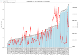
- The graph below shows the average SSIM for each stock ticker across all other stock price series.
- I pre-train the model with SICPQ (high gap), CUBI (medium gap) and RF (stable) and evaluate with SIVBQ (high gap), WAL (medium gap), RF (stable)
Week 18:
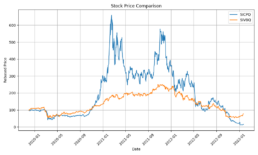
- I think the behaviour of the most interesting stock pair time series for the period 2020-2023 in the dataset is SIVBQ and SICPQ. However, their performance difference is significant. I can train the model to reach a training loss rate < 0.001 and R^2 0.9978 but the evaluation dataset r^2 remains around zero. Regularization techniques do not help due to the differences between these two time series.
- I have considered training the model for one of these two stocks and then fine-tune it to the other stock. However I would need to find a somehow similar stock time series because none of the stocks in my existing dataset is similar. I could indeed look further into this option. However I find more interesting to research the application of domain-informed data augmentation by transforming the training time series to include noise, shifts and trends observed in the evaluation data, or the generation of a synthetic timeseries with Variational Autoencoders.
Backlog
- Pre-processing/Transformations:
- Test AIMv2 SSIM for image/embeddings relational properties and quality of embeddings since pytorch ssim validates that the visual structure of input images has been retained
- refactor:
- batch regularization dynamic calc for group# depending on arch complexity
- tie out use_adaptiveAvgPool2d
- drop in GPU performance due to evaluation during training
- mlflow log_metrics end of batch and end of epoch with corresponding dict
- code new mlflow model storage
- parameters input to freeze the selection of layers
- create script to delete from db deleted experiments but first undelete run_17-11-2024 22:47:57
- Encode images accounting for gamma
- Since it’s likely the dataset’s max-min is large and the data volatile, differencing transformation (i.e. abs % change) is unlikely to help the model on its learning, but we’ll test it.
- Embeddings – leaning towards stumpy library for matrix profiles with interesting applications.
- Refactor mlflow warning UCVolumeDatasetSource
- Implement DTW with RAPIDS cuML as fastdtw lib runs on CPU
- Test AIMv2 SSIM for image/embeddings relational properties and quality of embeddings since pytorch ssim validates that the visual structure of input images has been retained
